How to Make a Trading Bot with Raspberry Pi?

The current popularity of cryptocurrencies also includes trading in them. Last year, I wrote an article How to automate your cryptocurrency trades with Python which covered the setup of a trading bot based on the graphical programming framework Pythonic, which I developed in my leisure. At that time, you still needed a desktop system based on x86 to run Pythonic. In the meantime, I have reconsidered the concept (web-based GUI). Today, it is possible to run Pythonic on a Raspberry Pi, which mainly benefits the power consumption because such a trading bot has to be constantly switched on.
That previous article is still valid. If you want to create a trading bot based on the old version of Pythonic (0.x), you can install it with pip3 install Pythonic==0.19.
This article covers the setup of a trading bot running on a Raspberry Pi and executing a trading algorithm based on the EMA crossover strategy.
Install Pythonic on your Raspberry Pi
Here, I only briefly touch on the subject of installation because you can find detailed installation instructions for Pythonic in my last article Control your Raspberry Pi remotely with your smartphone. In a nutshell: Download the Raspberry Pi image from sourceforge.net and flash it on the SD card.
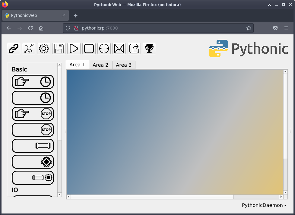
The PythonicRPI image has no preinstalled graphical desktop, so to proceed, you should be able to access the programming web GUI (http : //PythonicRPI:7000/):
(Stephan Avenwedde, CC BY-SA 4.0)
Example code
Download the example code for the trading bot from GitHub (direct download link) and unzip the archive. The archive contains three different file types:
\*.py-files: Contains the actual implementation of certain functionalitycurrent_config.json: This file describes the configured elements, the links between the elements, and the variable configuration of elementsjupyter/backtest.ipynb: A Jupyter notebook for backtestingjupyter/ADAUSD_5m.df: A minimal OHLCV dataset which I use in this example
With the green outlined button, upload the current_config.json to the Raspberry Pi. You can upload only valid configuration files. With the yellow outlined button, upload all the \*.py files.

(Stephan Avenwedde, CC BY-SA 4.0)
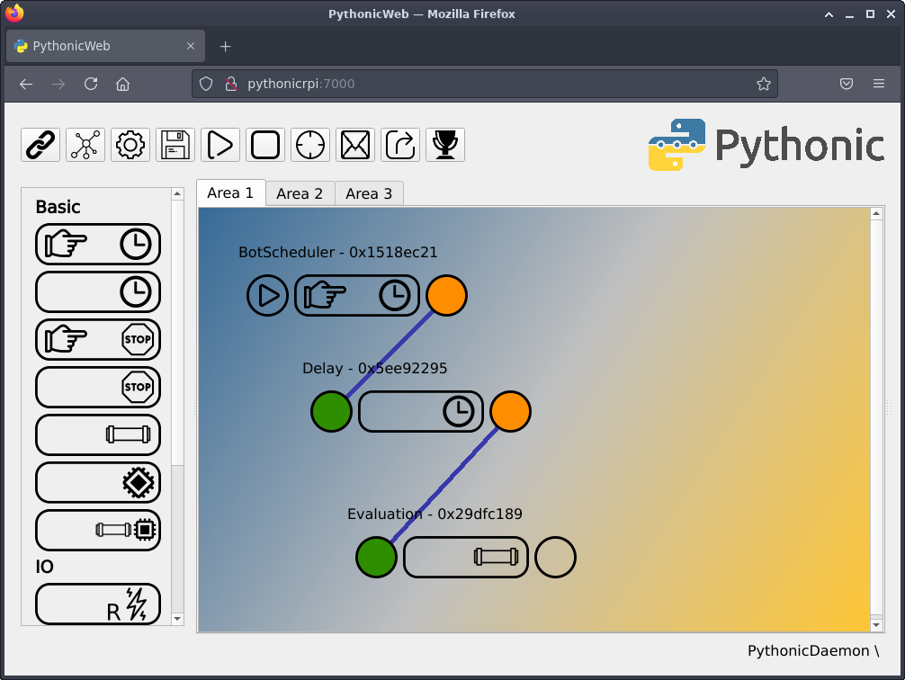
The \*.py files are uploaded to /home/pythonic/Pythonic/executables whereas the current_config.json is uploaded to /home/pythonic/Pythonic/current_config.json. After uploading the current_config.json, you should see a screen like this:
(Stephan Avenwedde, CC BY-SA 4.0)
Now I’ll go step-by-step through each part of the trading bot.
Data acquisition
Like in the last article, I begin with the data acquisition:
(Stephan Avenwedde, CC BY-SA 4.0)
More on Raspberry Pi
- What is Raspberry Pi?
- eBook: Guide to Raspberry Pi
- Getting started with Raspberry Pi cheat sheet
- eBook: Running Kubernetes on your Raspberry Pi
- Whitepaper: Data-intensive intelligent applications in a hybrid cloud blueprint
- Understanding edge computing
- Our latest on Raspberry Pi
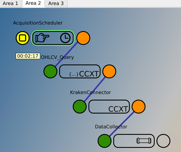
The data acquisition can be found on the Area 2 tab and runs independently from the rest of the bot. It implements the following functionality:
- AcqusitionScheduler: Trigger subsequent elements every five minutes
- OHLCV_Query: Prepares the OHLCV query method
- KrakenConnector: Establishes a connection with the Kraken cryptocurrency exchange
- DataCollector: Collect and process the new OHLCV data
The DataCollector gets a Python list of OHLCV data with a prefixed timestamp and converts it into a Pandas DataFrame. Pandas is a popular library for data analysis and manipulation. A DataFrame is the base type for data of any kind to which arithmetic operation can be applied.
The task of the DataCollector (generic_pipe_3e059017.py) is to load an existing DataFrame from file, append the latest OHLCV data, and save it back to file.
import time, queue
import pandas as pd
from pathlib import Path

try:
    from element_types import Record, Function, ProcCMD, GuiCMD
except ImportError:
    from Pythonic.element_types import Record, Function, ProcCMD, GuiCMD

class Element(Function):

    def __init__(self, id, config, inputData, return_queue, cmd_queue):
        super().__init__(id, config, inputData, return_queue, cmd_queue)

    def execute(self):
        df_in = pd.DataFrame(self.inputData, columns=['close_time', 'open', 'high', 'low', 'close', 'volume'])
        df_in['close_time'] = df_in['close_time'].floordiv(1000) # remove milliseconds from timestamp

        file_path = Path.home() / 'Pythonic' / 'executables' / 'ADAUSD_5m.df'

        try:
            # load existing dataframe
            df = pd.read_pickle(file_path)
            # count existing rows
            n_row_cnt = df.shape[0]
            # concat latest OHLCV data
            df = pd.concat([df,df_in], ignore_index=True).drop_duplicates(['close_time'])
            # reset the index
            df.reset_index(drop=True, inplace=True)
            # calculate number of new rows
            n_new_rows = df.shape[0] - n_row_cnt
            log_txt = '{}: {} new rows written'.format(file_path, n_new_rows)

        except Exception as e:
            log_txt = 'File error - writing new one'
            df = df_in

        # save dataframe to file
        df.to_pickle(file_path)

        logInfo = Record(None, log_txt)
        self.return_queue.put(logInfo)
This code is executed every full five minutes as the OHLCV data is also in 5-minute intervals.
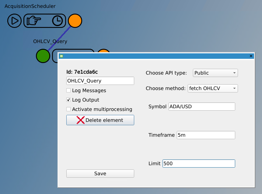
By default, the OHLCV_Query element only downloads the dataset for the latest period. To have some data for developing the trading algorithm, right-click the OHLCV_Query element to open the configuration, set the Limit to 500, and trigger the AcquisitionScheduler. This causes the download of 500 OHLCV values:
(Stephan Avenwedde, CC BY-SA 4.0)
Trading strategy
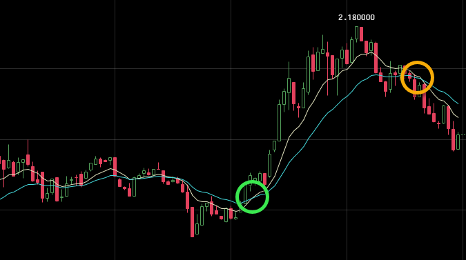
Our trading strategy will be the popular EMA crossover strategy. The EMA indicator is a weighted moving average over the last n close prices that gives more weight to recent price data. You calculate two EMA series, one for a longer period (for example, n = 21, blue line) and one for a shorter period (for example, n = 10, yellow line).
(Stephan Avenwedde, CC BY-SA 4.0)
The bot should place a buy order (green circle) when the shorter-term EMA crosses above the longer-term EMA. The bot should place a sell order when the shorter-term EMA crosses below the longer-term EMA (orange circle).
Backtesting with Jupyter
The example code on GitHub (direct download link) also contains a Jupyter Notebook file (backtesting.ipynb) which you use to test and develop the trading algorithm.
Note: Jupyter is not preinstalled on the Pythonic Raspberry Pi image. You can either install it also on the Raspberry Pi or install it on your regular PC. I recommend the latter, as you will do some number crunching that is much faster on an ordinary x86 CPU.
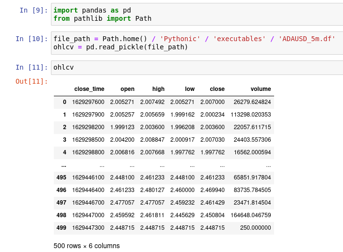
Start Jupyter and open the notebook. Make sure to have a DataFrame, downloaded by the DataCollector, available. With Shift+Enter, you can execute each cell individually. After executing the first three cells, you should get an output like this:
(Stephan Avenwedde, CC BY-SA 4.0)
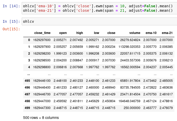
Now calculate the EMA-10 and EMA-21 values. Luckily, pandas offers you the ewm function, which does exactly what is needed. The EMA values are added as separate columns to the DataFrame:
(Stephan Avenwedde, CC BY-SA 4.0)
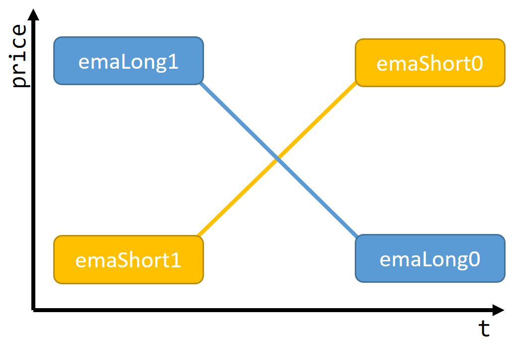
To determine if a buy or sell condition is met, you have to consider these four variables:
- emaLong0: Current long-term (ema-21) EMA value
- emaLong1: Last long-term (ema-21) EMA value (the value before emaLong0)
- emaShort0: Current short-term (ema-10) EMA value
- emaShort1: Last short-term (ema-10) EMA value (the value before emaShort0)
When the following situation comes into effect, a buy condition is met:
(Stephan Avenwedde, CC BY-SA 4.0)
In Python code:
emaLong1 > emaShort1 and emaShort0 > emaLong0A sell condition is met in the following situation:
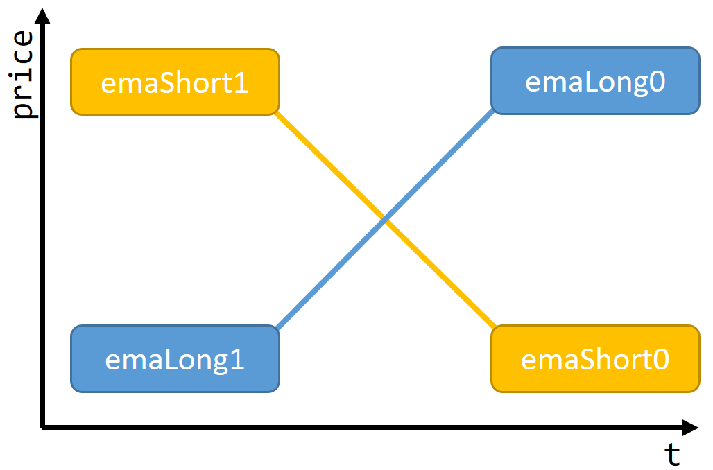
(Stephan Avenwedde, CC BY-SA 4.0)
In Python code:
emaShort1 > emaLong1 and emaLong0 > emaShort0To test the DataFrame and evaluate the possible profit you could make, you could either iterate over each row and test for these conditions or, with a smarter approach, filter the dataset to only the relevant rows with built-in methods from Pandas.
Under the hood, Pandas uses NumPy, which is the method of choice for fast and efficient data operation on arrays. This is, of course, convenient because the later use is to take place on a Raspberry Pi with an ARM CPU.
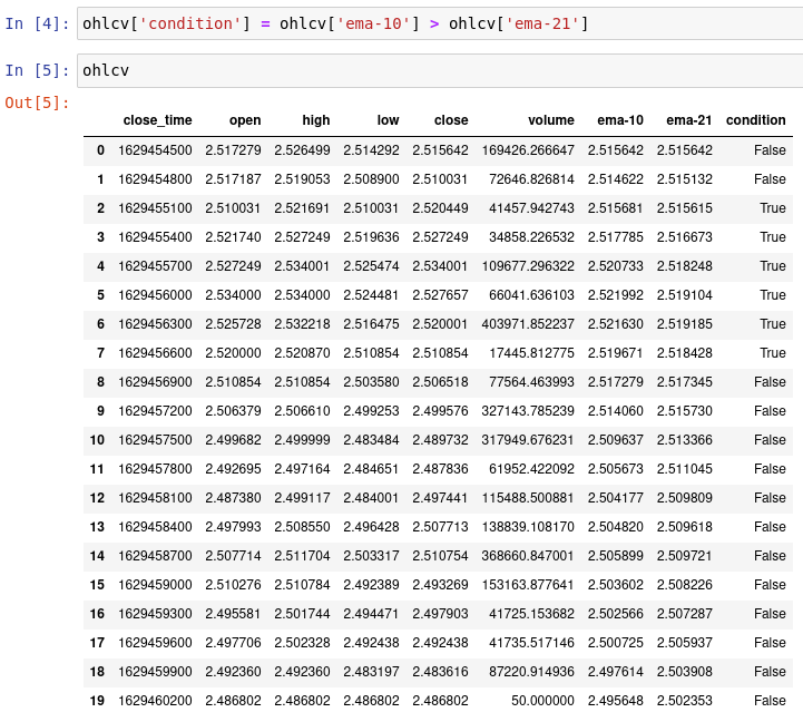
For the sake of clarity, the DataFrame from the example (ADAUSD_5m.df) with only 20 entries is used in the following examples. The following code appends a column of boolean values dependent on the condition emaShort0 > emaLong0:
(Stephan Avenwedde, CC BY-SA 4.0)
The place of interest is when a False switches to True (buy) or when True switches to False. To filter them apply a diff operation to the condition column. The diff operation calculates the difference between the current and the previous line. In terms of boolean values, it results in:
- False
diffFalse = False - False
diffTrue = True - True
diffTrue = False - True
diffFalse = True
With the following code, you apply the diff operation as a filter to the condition column without modifying it:

(Stephan Avenwedde, CC BY-SA 4.0)
As a result, you get the desired data: The first row (index 2) signalizes a buy condition and the second row (index 8) signalizes a sell condition. As you now have an efficient way of extracting relevant data, you can calculate possible profit.
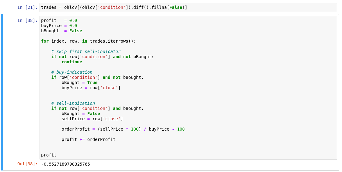
To do so, you have to iterate through the rows and calculate the possible profit based on simulated trades. The variable bBought saves the state if you already bought, and buyPrice stores the price you bought between the iterations. You also skip the first sell indicator as it doesn’t make sense to sell before you’ve even bought.
profit   = 0.0
buyPrice = 0.0
bBought  = False

for index, row, in trades.iterrows():

    # skip first sell-indicator
    if not row['condition'] and not bBought:
        continue

    # buy-indication
    if row['condition'] and not bBought:
        bBought = True
        buyPrice = row['close']


    # sell-indication
    if not row['condition'] and bBought:
        bBought = False
        sellPrice = row['close']

        orderProfit = (sellPrice * 100) / buyPrice - 100

        profit += orderProfit
Your one-trade mini dataset would provide you the following profit:
(Stephan Avenwedde, CC BY-SA 4.0)
Note: As you can see, the strategy would have given a terrible result as you would have bought at $2.5204 and sold at $2.5065, causing a loss of 0.55% (order fees not included). However, this is a real-world scenario: One strategy does not work for each scenario. It is on you to find the most promising parameters (for example, using OHLCV on an hourly basis would make more sense in general).
Implementation
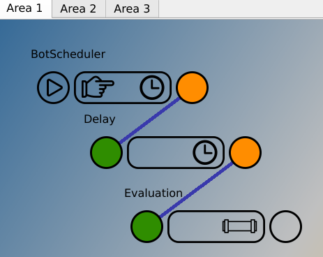
You can find the implementation of the decision on the Area 1 tab.
(Stephan Avenwedde, CC BY-SA 4.0)
It implements the following functionality:
- BotScheduler: Same as the AcqusitionScheduler: Trigger subsequent elements every five minutes
- Delay: Delay the execution for 30 seconds to make sure that the latest OHLCV data was written to file
- Evaluation: Make the trading decision based on the EMA crossover strategy
You now know how the decision makings work, so you can take a look at the actual implementation. Open the file generic_pipe_29dfc189.py. It corresponds to the Evaluation element on the screen:
@dataclass
class OrderRecord:
    orderType:          bool  # True = Buy, False = Sell
    price:              float # close price
    profit:             float # profit in percent
    profitCumulative:   float # cumulative profit in percent


class OrderType(Enum):
    Buy  = True
    Sell = False


class Element(Function):

    def __init__(self, id, config, inputData, return_queue, cmd_queue):
        super().__init__(id, config, inputData, return_queue, cmd_queue)

    def execute(self):

        ### Load data ###

        file_path = Path.home() / 'Pythonic' / 'executables' / 'ADAUSD_5m.df'

        # only the last 21 columsn are considered
        self.ohlcv = pd.read_pickle(file_path)[-21:]

        self.bBought             = False
        self.lastPrice           = 0.0
        self.profit              = 0.0
        self.profitCumulative    = 0.0
        self.price               = self.ohlcv['close'].iloc[-1]

        # switches for simulation

        self.bForceBuy  = False
        self.bForceSell = False

        # load trade history from file
        self.trackRecord = ListPersist('track_record')

        try:
            lastOrder = self.trackRecord[-1]

            self.bBought          = lastOrder.orderType
            self.lastPrice        = lastOrder.price
            self.profitCumulative = lastOrder.profitCumulative

        except IndexError:
            pass

        ### Calculate indicators ###

        self.ohlcv['ema-10'] = self.ohlcv['close'].ewm(span = 10, adjust=False).mean()
        self.ohlcv['ema-21'] = self.ohlcv['close'].ewm(span = 21, adjust=False).mean()
        self.ohlcv['condition'] = self.ohlcv['ema-10'] > self.ohlcv['ema-21']

        ### Check for Buy- / Sell-condition ###
        tradeCondition = self.ohlcv['condition'].iloc[-1] != self.ohlcv['condition'].iloc[-2]

        if tradeCondition or self.bForceBuy or self.bForceSell:

            orderType = self.ohlcv['condition'].iloc[-1] # True = BUY, False = SELL

            if orderType and not self.bBought or self.bForceBuy: # place a buy order

                msg         = 'Placing a  Buy-order'
                newOrder    = self.createOrder(True)

            elif not orderType and self.bBought or self.bForceSell: # place a sell order

                msg = 'Placing a  Sell-order'

                sellPrice   = self.price
                buyPrice    = self.lastPrice

                self.profit = (sellPrice * 100) / buyPrice - 100
                self.profitCumulative += self.profit

                newOrder = self.createOrder(False)

            else: # Something went wrong
                msg = 'Warning: Condition for {}-order met but bBought is {}'.format(OrderType(orderType).name, self.bBought)
                newOrder = None


            recordDone = Record(newOrder, msg)
            self.return_queue.put(recordDone)

    def createOrder(self, orderType: bool) -> OrderRecord:

        newOrder = OrderRecord(
                orderType=orderType,
                price=self.price,
                profit=self.profit,
                profitCumulative=self.profitCumulative
            )

        self.trackRecord.append(newOrder)

        return newOrder
As the general process is not that complicated, I want to highlight some of the peculiarities:
Input data
The trading bot only processes the last 21 elements as this is the range you consider when calculating the exponential moving average:
self.ohlcv = pd.read_pickle(file_path)[-21:]Track record
The type ListPersist is an extended Python list object that writes itself to the file system when modified (when elements get added or removed). It creates the file track_record.obj under ~/Pythonic/executables/ once you run it the first time.
self.trackRecord = ListPersist('track_record')Maintaining a track record helps to keep the state of recent bot activity.
Plausibility
The algorithm outputs an object of the type OrderRecord in case conditions for a trade are met. It also keeps track of the overall situation: For example, if a buy signal was received, but bBought indicates that you already bought before, something must’ve gone wrong:
else: # Something went wrong
    msg = 'Warning: Condition for {}-order met but bBought is {}'.format(OrderType(orderType).name, self.bBought)
    newOrder = None
In this scenario, None is returned with a corresponding log message.
Simulation
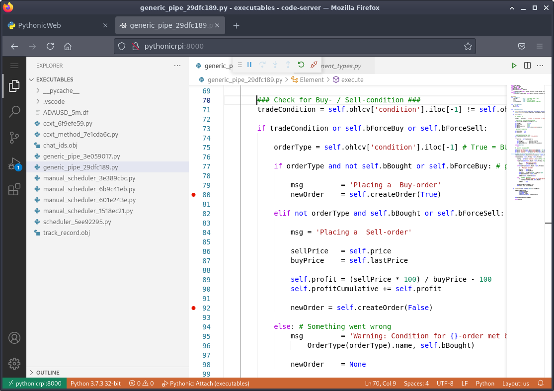
The Evaluation element (generic_pipe_29dfc189.py) contains these switches which enable you to force the execution of a buy or sell order:
self.bForceBuy  = False
self.bForceSell = False
Open the code server IDE (http : //PythonicRPI:8000/), load generic_pipe_29dfc189.py and set one of the switches to True. Attach with the debugger and add a breakpoint where the execution path enters the inner if conditions.
(Stephan Avenwedde, CC BY-SA 4.0)
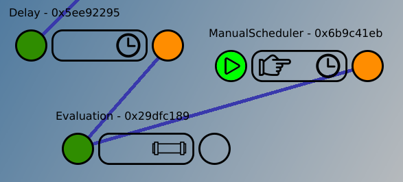
Now open the programming GUI, add a ManualScheduler element (configured to single fire) and connect it directly to the Evaluation element to trigger it manually:
(Stephan Avenwedde, CC BY-SA 4.0)
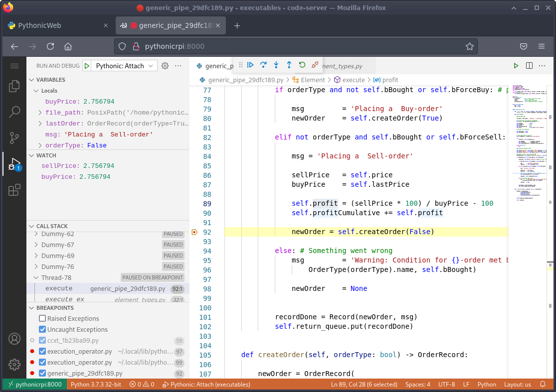
Click the play button. The Evaluation element is triggered directly, and the debugger stops at the previously set breakpoint. You are now able to add, remove, or modify orders from the track record manually to simulate certain scenarios:
(Stephan Avenwedde, CC BY-SA 4.0)
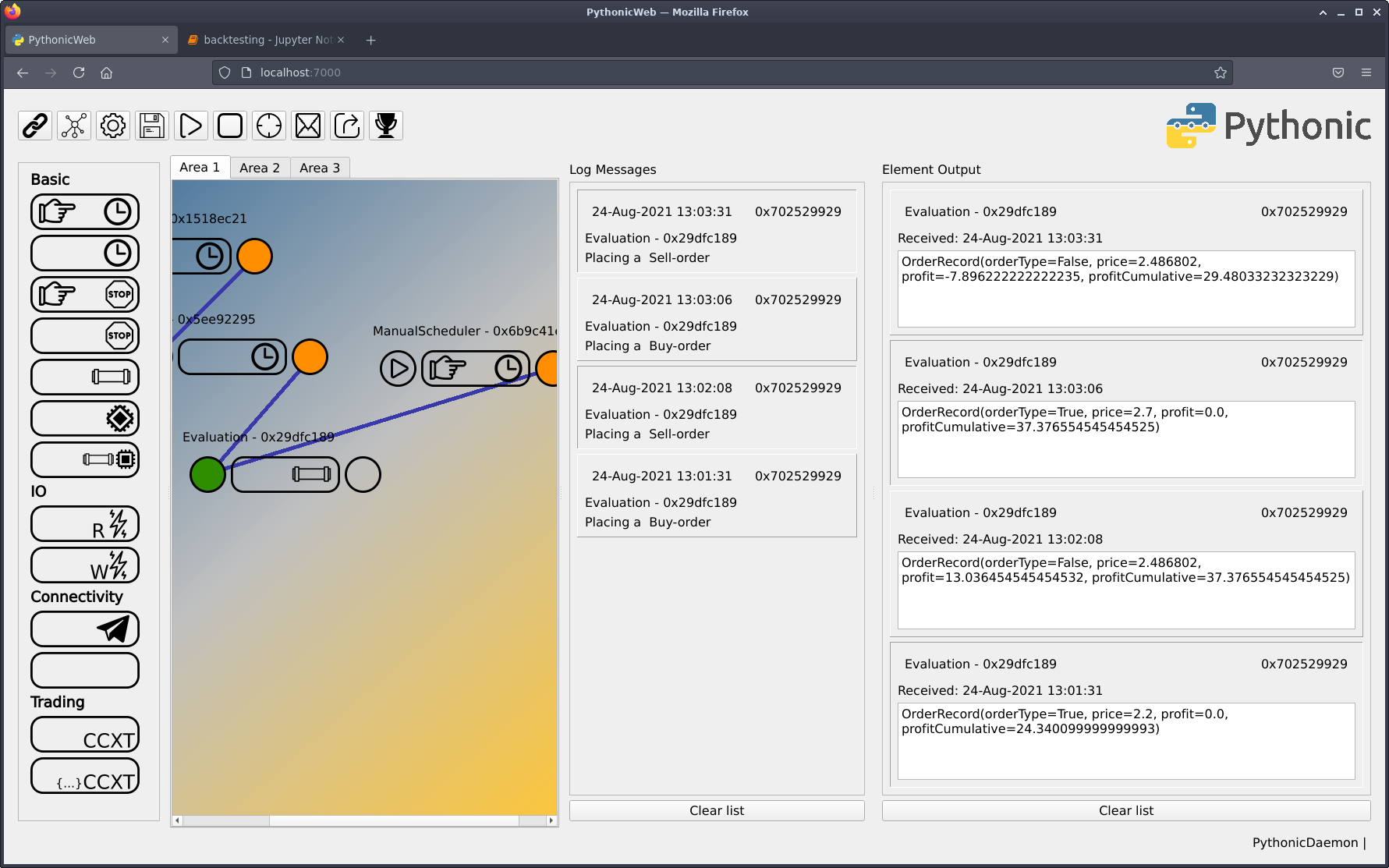
Open the log message window (green outlined button) and the output data window (orange outlined button):

(Stephan Avenwedde, CC BY-SA 4.0)
You will see the log messages and output of the Evaluation element and thus the behavior of the decision-making algorithm based on your input:
 (Stephan Avenwedde, CC BY-SA 4.0)
Summary
The example stops here. The final implementation could notify the user about a trade indication, place an order on an exchange, or query the account balance in advance. At this point, you should feel that everything connects and be able to proceed on your own.
Using Pythonic as a base for your trading bot is a good choice because it runs on a Raspberry Pi, is entirely accessible by a web browser, and already has logging features. It is even possible to stop on a breakpoint without disturbing the execution of other tasks using Pythonic’s multiprocessing capabilities.

 (Stephan Avenwedde,